Site response of a soil layer: a finite difference model verified against the closed-form solution
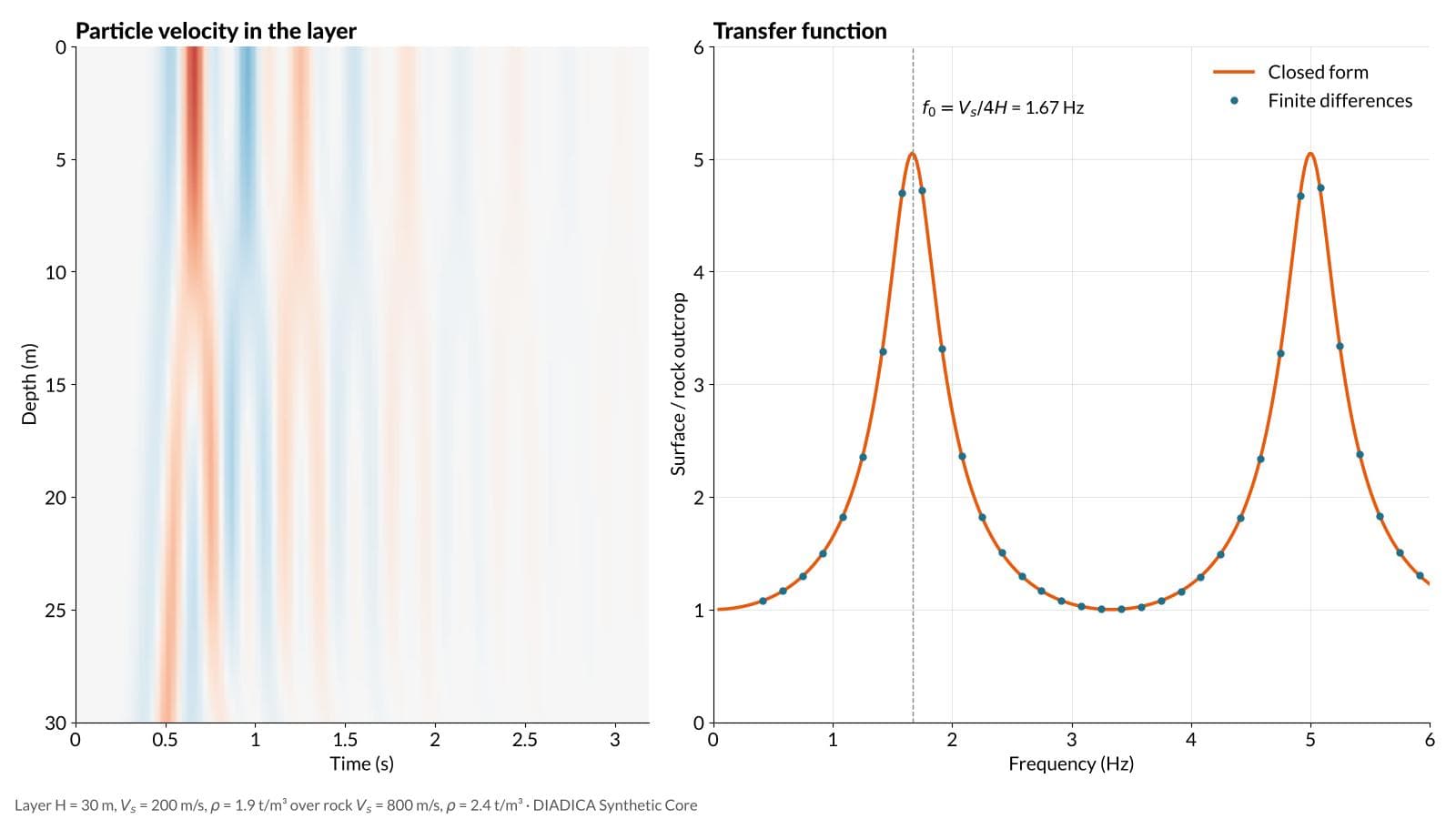
Shear wave propagation in a 30 m layer over rock, solved by finite differences and checked against the theoretical transfer function. The model reproduces the 1.67 Hz fundamental frequency and the 5.05 amplification with a maximum error of 0.17%.
Amplification of seismic waves in a soil deposit is one of the effects that changes the demand on a structure the most. NSR-10 includes it in the design spectrum through the site coefficients Fa and Fv, which summarize the behaviour of families of profiles. When a profile falls outside those families, or the project requires a site-specific study, the response is computed with a model of the deposit, and before that model is used it has to be shown that it solves the wave equation correctly. This note presents that check on the simplest case that has a closed-form solution.
The reference case
A homogeneous layer of H = 30 m is analysed, with shear wave velocity Vs = 200 m/s and density ρ = 1.9 t/m³, resting on rock with Vr = 800 m/s and ρr = 2.4 t/m³. For a shear wave arriving vertically from the rock, the ratio between the motion at the surface of the layer and that of the rock outcrop is
|A(f)| = 1 / √( cos²(kH) + α² sin²(kH) ), with k = 2πf / Vs and α = ρVs / (ρrVr)
With the data of the case, the impedance ratio is α = 0.198. The peaks of the function occur at fn = (2n − 1)Vs/4H, that is 1.67 Hz for the fundamental mode and 5.00 Hz for the second, and without damping their value is 1/α = 5.05.
The numerical model
The one-dimensional wave equation was solved in Python with explicit finite differences, using 300 elements of 0.10 m and a time step of 0.2 ms, which corresponds to a Courant number of 0.4. The surface is modelled as a stress-free boundary. At the base a Lysmer transmitting boundary introduces the incident wave and lets the reflected energy leave into the rock; its dashpot is treated implicitly so the scheme remains stable with that time step. The excitation is a 3 Hz Ricker pulse and 12 s of response are simulated.
The numerical transfer function is obtained as the ratio between the Fourier spectra of the surface velocity and of twice the incident wave, which is the motion of the rock outcrop.
Results
The model places the first peak at 1.665 Hz with an amplitude of 5.053, against 1.664 Hz and 5.052 for the closed-form solution. The second peak appears at 4.996 Hz with an amplitude of 5.052. Over the whole band between 0.3 and 6 Hz the maximum relative error with respect to the theoretical solution is 0.17%, and in the band of the fundamental mode it is 0.08%.
The figure shows on the left how the pulse travels up the layer, reflects at the surface and is trapped by the impedance contrast, and on the right the numerical transfer function over the theoretical one.
Scope
The case has neither damping nor soil nonlinearity, so the amplification of 5.05 is an upper value. With hysteretic damping ξ the peak of the fundamental mode drops to approximately 1/(α + πξ/2); for ξ = 5% the value becomes 3.6. Equivalent linear and nonlinear analyses start from this same scheme, with strain-dependent properties, and they only make sense on a numerical engine that has already reproduced the elastic case.
This exercise is part of the verification cases of DIADICA Synthetic Core in computational geotechnics, and it is also one of the examples solved in the DIADICA Academy courses.