Synthetic Core · Simulators
Engineering simulators
Problems in geotechnics, structural steel, hydrogeology, air quality and seismic analysis, solved in the browser or with precomputed models. Each result is compared with a second method, an analytical solution or a published benchmark, and the difference is reported.
Comparison of two methods
Problems solved with two methods based on independent assumptions, with the difference between the two results.
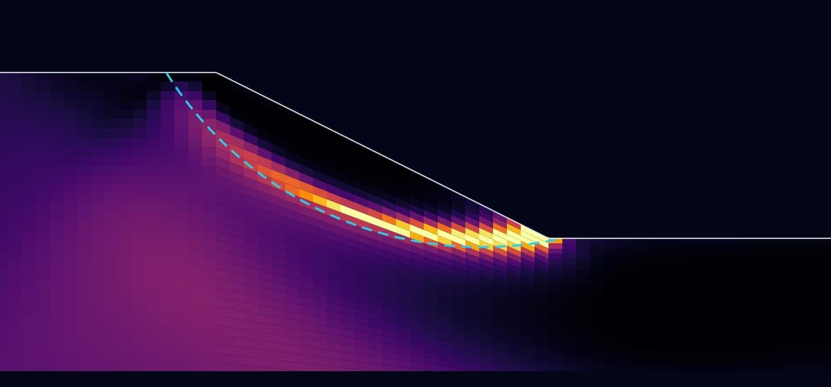
Simplified Bishop, finite elements and ACADS benchmarks
Slope stability
Limit equilibrium is computed in the browser from the input data. The finite element model forms the failure band without an imposed surface, and the ACADS cases check it against a published benchmark.
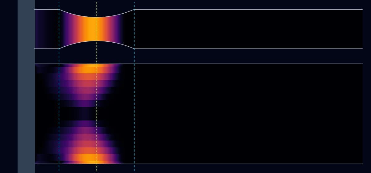
AISC 358 and finite elements with von Mises plasticity
Reduced beam section (RBS) moment connection
The beam is taken to a rotation of 0.05 rad without imposing the location of yielding. The moment and the hinge position are compared with the assumptions of AISC 358.
Against a reference solution
Numerical models compared with an analytical solution or a published benchmark.
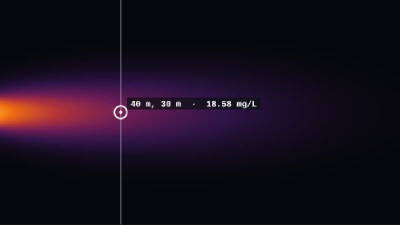
Finite differences with advection, dispersion and decay
Contaminant transport in groundwater
Advance of the plume through the aquifer with a movable monitoring well that records the concentration, overlaid on the analytical solution.
Domenico (1987): maximum difference 4.6 % of c₀
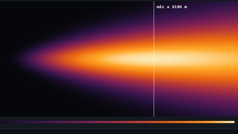
Gaussian plume with sensitivity analysis
Atmospheric pollutant dispersion
Ground-level concentration by atmospheric stability, stack height and wind. The same problem is solved three ways: closed form, numerical integration and mass balance.
Three independent routes: difference below 0.06 %
Closed-form solutions
Code or mechanics equations presented with their input, so the result can be reproduced by hand.
Simulation Mode
Run each simulator on its own or apply the same intensity to all three.
System Inputs
Parameters applied at once to the three simulators. The intensity sets the demand of each one: Aa = Av from 0.10 to 0.40 for the building, P from 0 to 4,000 kN for the footing and P/Pn from 0 to 100 % for the column.
Structural Response Simulator
Equivalent Lateral Force, NSR-10
Approximate period, design spectrum, base shear and its distribution over height, with a spectral estimate of drift against the 1.0 % h limit.
Parameters
Spectrum (soil D, I = 1.0)
Equivalent lateral force
Lateral displacement u(z) [mm]
Storey shear Vx [kN]
Displacement (approximate)
Maximum drift
NSR-10 A.6.4 limit: 1.0 % h
Model scope: NSR-10 equivalent lateral force method (A.2 and A.4) with T = Ta, soil type D (Fa and Fv interpolated from tables A.2.4-3 and A.2.4-4), Av = Aa and I = 1.0. Seismic weight 10 kN/m² over 300 m² per storey and 3.0 m storey height. Displacement is a spectral estimate: Γ = 1.3, linear shape for frames and parabolic for walls; it does not replace the analysis of the model.
Soil-Structure Interaction Simulator
Stress Bulb & Elastic Settlement
Vertical stress increase under a square footing from Newmark’s solution and immediate settlement on an elastic half-space.
Load and geometry
Soil and footing
Results
Stress bulb Δσz/q (vertical section through the centre)
Superposition of Newmark’s solution for a loaded rectangle. Domain: 4B wide by 3B deep. The white line is the Δσz = 0.1q contour.
Model scope: Square footing on an elastic, homogeneous, isotropic half-space under uniform pressure q. Stresses from integrated Boussinesq (Newmark); immediate elastic settlement, no consolidation and no embedment correction.
Column Buckling Simulator
Compressive Strength & Imperfection Amplification
Critical stress per AISC 360-16 chapter E (NSR-10 F.2.5) and amplification of the initial deflection δ0/(1 − P/Pe) in a pin-ended column.
Input Parameters
Results
Deflected shape of the pin-ended column (lateral scale ×40)
Fcr vs. KL/r curve
Model scope: Pin-ended W8×31 column (Ag = 5,890 mm², ry = 51.3 mm), A572 Gr. 50 steel, Fy = 345 MPa, E = 200,000 MPa. Nominal strength per AISC 360-16 section E3 (NSR-10 F.2.5.3). Deflection uses the elastic amplification of a sinusoidal imperfection δ0; residual stresses and section yielding are not included.
Use. Demonstration material, not for design. Application to a project and the calculation notebook are reviewed in a technical meeting.
Book a demonstration